How TO Land an Orbital Rocket Booster: a gentle mathematical introduction

With terminal-phase Guidance Navigation and Control in the news lately with the (qualified) success of Intuitive Machines and JAXA’s lunar landers, I wanted to provide an approachable look at the mathematics of rocket landing, and the ways it’s both easier and harder than you might expect.

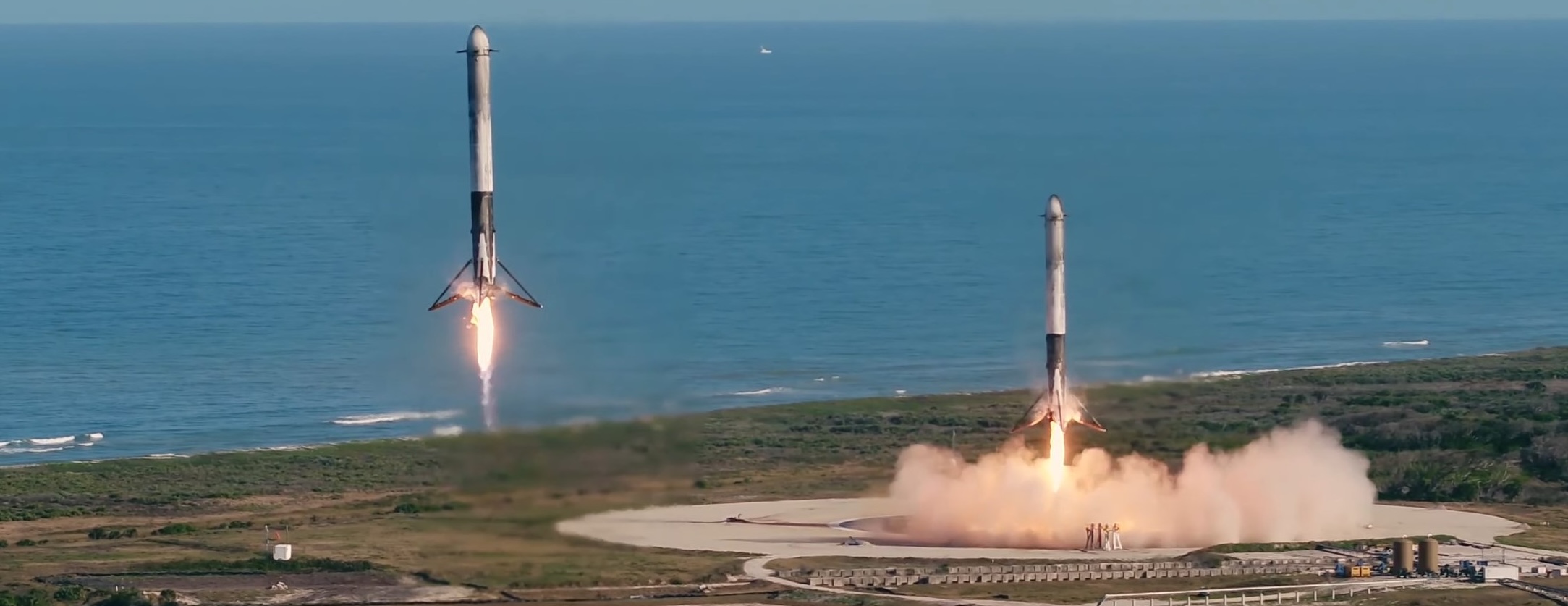
To me, there’s nothing more awe-inspiring than watching rockets land autonomously, and in fact watching this as a college freshman with the rocketry team was what inspired me to become a Guidance Navigation and Control (GN&C) Engineer in the first place.¹

But trajectory optimization and GN&C in general is notoriously math heavy and intimidating to learn - any primer on the subject I’ve encountered online either brushes over the math entirely (“the rocket uses grid fins for control”) or mentions semidefinite matrices within the first two paragraphs. For a beginner genuinely interested in the subject, neither is ideal.

In this post, I aim to provide a gentle (~calculus-level) introduction to the math behind these problems - what is the intuition for the solution methods, how do they work in practice, and what makes this problem so hard anyway?

1. Historical Approaches

The problem of controlling a spacecraft in space is relatively easy² up until the landing attempt - in space, things mostly do what you tell them to do. Other than gravity, there are no pesky “atmospheres” or “solid items” to run into and knock you off course. This is an engineers dream - in space, every cow is spherical.

This changes once you attempt to land on the surface - not only are there a variety of disturbances to contend with (poorly modeled atmospheres, wind, etc.), but things are much more high stakes - with every second, the spacecraft gets closer and closer to a rather prominent solid item named “the ground.”

We’ve been doing planetary landings for a few decades, and a few clear strategies have emerged:

Landing Strategy	Description	Pros	Cons	Notable Missions
Landing bags	Deploy massive airbags and bounce off the surface	-Relatively simple	-High deceleration loads -Imprecise landing zone	-Luna 9 in 1966, the first ever planetary soft landing -Several Mars rovers (Sojourner, Opportunity)
Piloted propulsive landing	Allow a human pilot to guide the spacecraft down manually	-Minimal algorithms required	-High risk -Does not apply to robotic missions	-Apollo 11 and others
Parachutes	Deploy parachutes to slow down craft before attempting propulsive or airbag landing	-Simple	-Needs an atmosphere -Not reusable	-Majority of missions to planets with atmospheres
Autonomous propulsive landing	Fire boosters backwards to minimize speed and land softly on the surface	-Completely reusable -High precision (in theory)	-Super hard!	-SpaceX booster landings on Earth -Perseverance Mars Rover -SLIM and IM-1 Lunar Missions

Many missions use a mixture of these approaches, but fully autonomous propulsive landing remains the holy grail - only this method promises pinpoint landing, full reusability, and high safety for hardware and humans.

Propulsive landing has been done in some form for decades, but there is still a large amount of room for improvement. In the words of the late Jim Martin, on the 1976 Viking mission, “[they] had no hazard avoidance whatsoever, just a lot of luck.” To meet the mission requirements of the future (including having humans aboard), we need algorithms that can achieve pinpoint landing on the surface, avoid obstacles, and adapt to changing circumstances on the fly.

While most recently Perserverance landed within 1km of it’s desired target, more accuracy is still desired and the performance of the recent SLIM and IM-1 missions make it clear that we have a long way to go for truly robust and efficient methods. This makes it, in my opinion, one of the clear open problems in aerospace engineering research today.

2. Problem Setup

Broadly, we care about getting a rocket from a starting location to the location of the landing site, with zero velocity³. Along the way, we likely have some secondary objectives, like minimizing fuel or time spent.

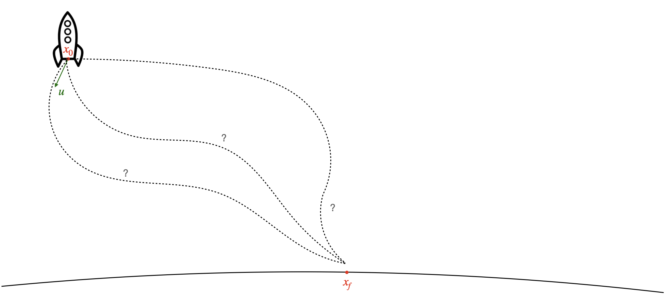
Typically, the position, velocity, and orientation of the rocket is represented by \(x\), called the “state” of the rocket. Similarly, we have some way of influencing the state of the rocket (i.e. a rocket engine), which we denote the “input” \(u\). Hopefully we also have an idea about how the position of the rocket will evolve over time according to the laws of physics and our input - in other words, we know some function \(f\) such that:

\[x_{k+1} = f(x_k, u_k)\]

This function could be as simple as a force pushing on a box in one dimension:

or as complicated as spacecraft rotational dynamics:

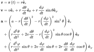
but the only thing that matters is that we can write this function down!⁴ Bringing this all together, mathematically, we can formulate a simple version of this problem as follows:⁵

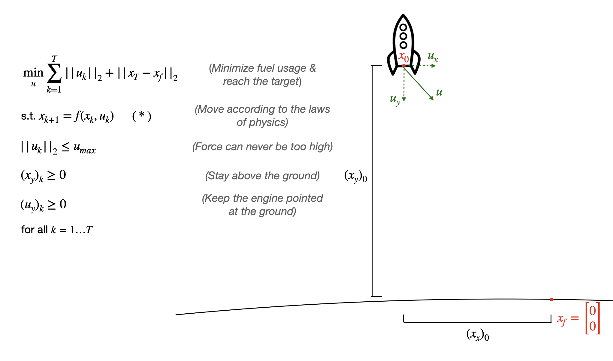
Although everything we’ve written down has a relatively simple motivation, looking at this as a human, this is a mess - how can you possibly come up with a sequence of \(u\)’s that gets you to your goal, let alone an optimal sequence, especially if \(f\) is a complicated function? Luckily, we have a way of doing this systematically which can be understood with little more math than is taught in high school calculus.

3. Sequential Convex Programming (SCP)

One of the primary enabling technologies of propulsive landing has been Sequential Convex Programming (SCP), which is a method of generating optimal solutions to problems of this type.

3.1. Convex Optimization Problems

One extremely important property of optimization problems is “convexity”. While we won’t get into the math here,⁶ the intuition is remarkably simple. Convex problems are shaped like bowls, where there is only one “local minimum”. This means that if you stop making progress, you know you’ve reached the optimal solution. By contrast, nonconvex problems can be arbitrarily shaped, and you can get stuck in a several places without knowing that if you try a bit harder, you can find an even better solution.

As a visual example, the function on the left below is convex, so if you roll a ball down the hill starting from anywhere, you’ll reach the minimum. For the nonconvex function on the right, the final location of the ball is dependent on where you start the ball. It’s not hard to see how this could translate to a tougher optimization problem.

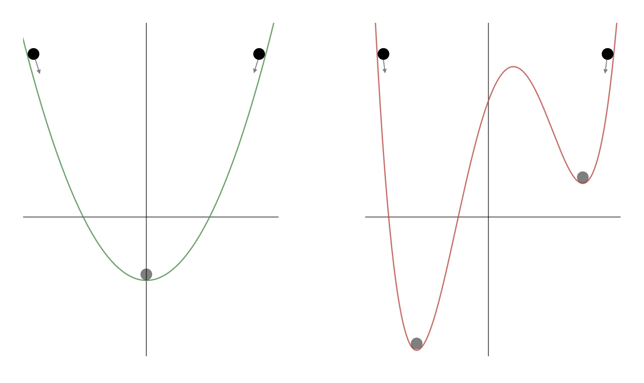
In the context of our rocket landing problem, fuel cost would be the y-axis. If we’re trying to find a trajectory with minimum fuel cost, the full problem might initially look like the plot on the right, which would make finding a minimum fuel cost very difficult. SCP allows us to approximate the problem on the right by solving problems that look like the plot on the left, making things much easier.⁷

Aside: Linearization
One key concept we need to develop in our discussion of successive convexification is linearization. Recall from calculus class that if we take the derivative of a function f(x) w.r.t x, plug in our point of interest x_0, and use that as the slope A of a new function, we can come up with an approximation to an arbitrarily complicated f(x) which is pretty good, as long as we're near our point x_0.

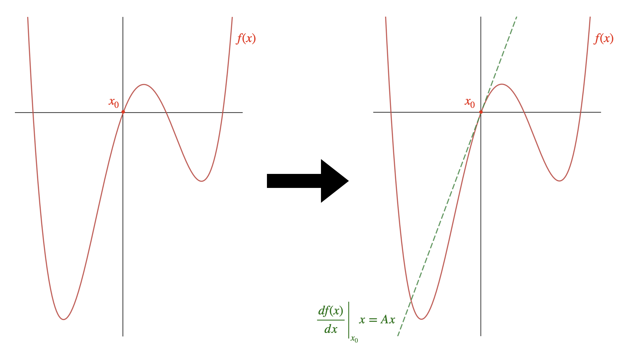
In the above example, we managed to replace our extremely complicated f(x), which has multiple local minima and maxima, with a MUCH simpler straight line, that performs basically the same way as long as we stay close to our linearization point x_0. This is a very simple way of "convexifying" our nonconvex dynamics so that we can optimize more efficiently.

3.2. The SCP Process

With an intuitive understanding of convex optimization, we can put it all together. The pseudocode of sequential convex programming is as follows:

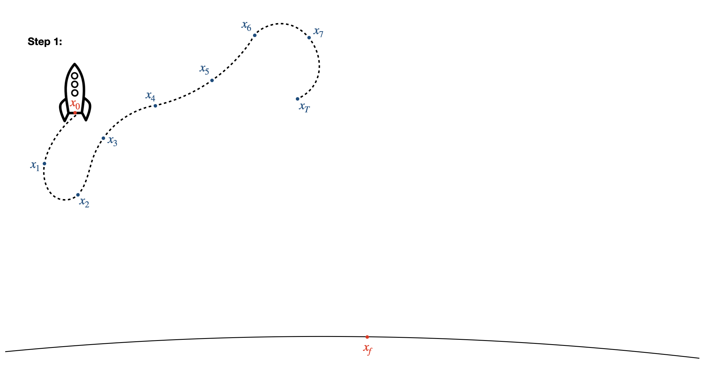
1. Starting from your initial condition \(x_0\), take a completely random guess at a sequence of inputs (for example - use \(u_k=0 \text{ for all } k=1...\ldots T\)). Use the dynamics function \(f(x,u)\) to calculate the state of the rocket at all times \(x_k\) based on these inputs.
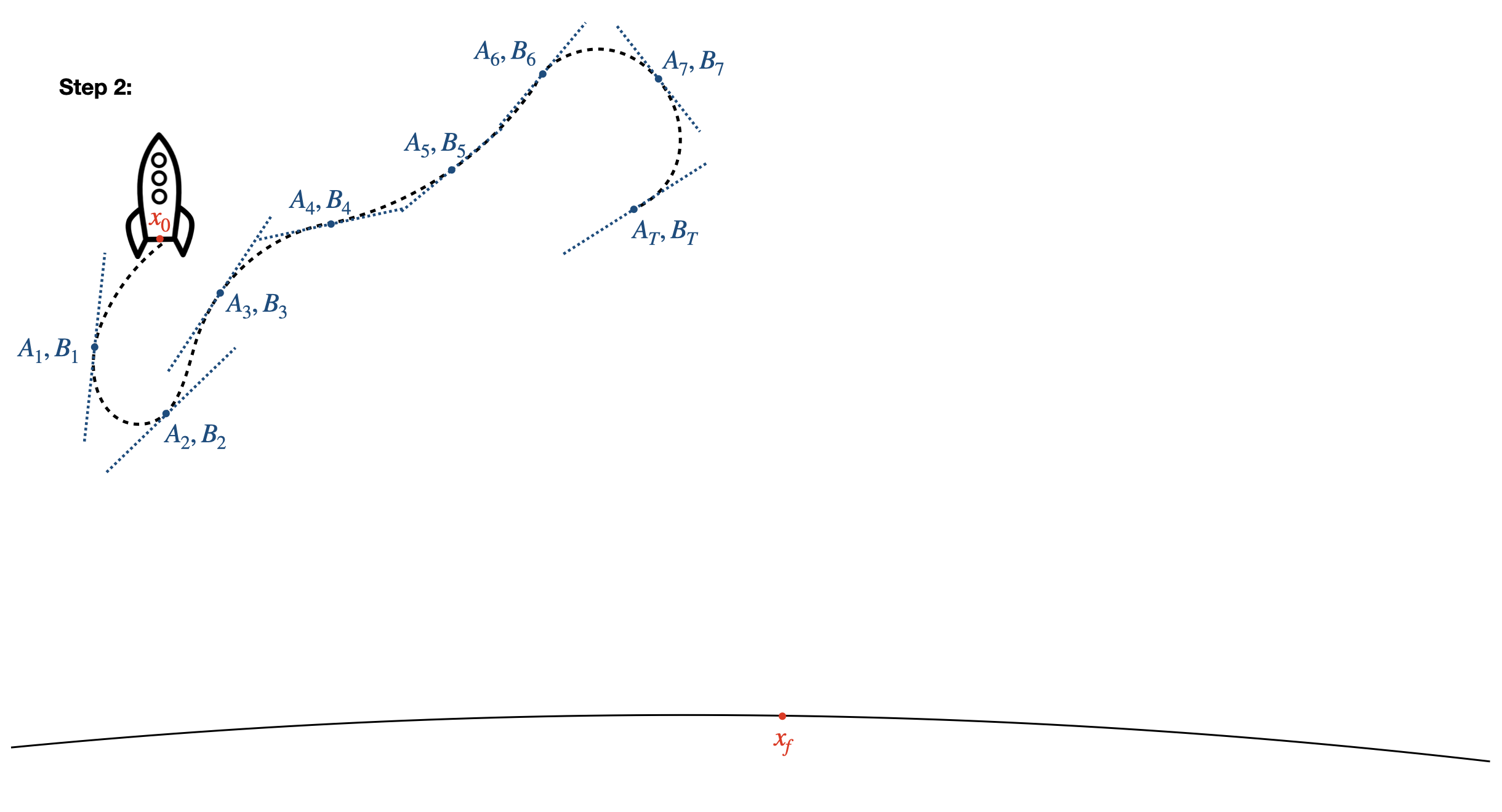
2. Approximate the dynamics by linearizing at every time step, \(x_{k+1} = A_k x_k + B_k u_k = \frac{df}{dx} \bigg \vert_{x_k} x_k + \frac{df}{du} \bigg \vert_{u_k} u_k\). Note that now, Equation \((*)\) is a convex constraint, so our optimization problem now looks like a bowl!
3. Solve the optimization problem using the linearized dynamics to ensure the problem is convex - this yields a new sequence of inputs \(u\).
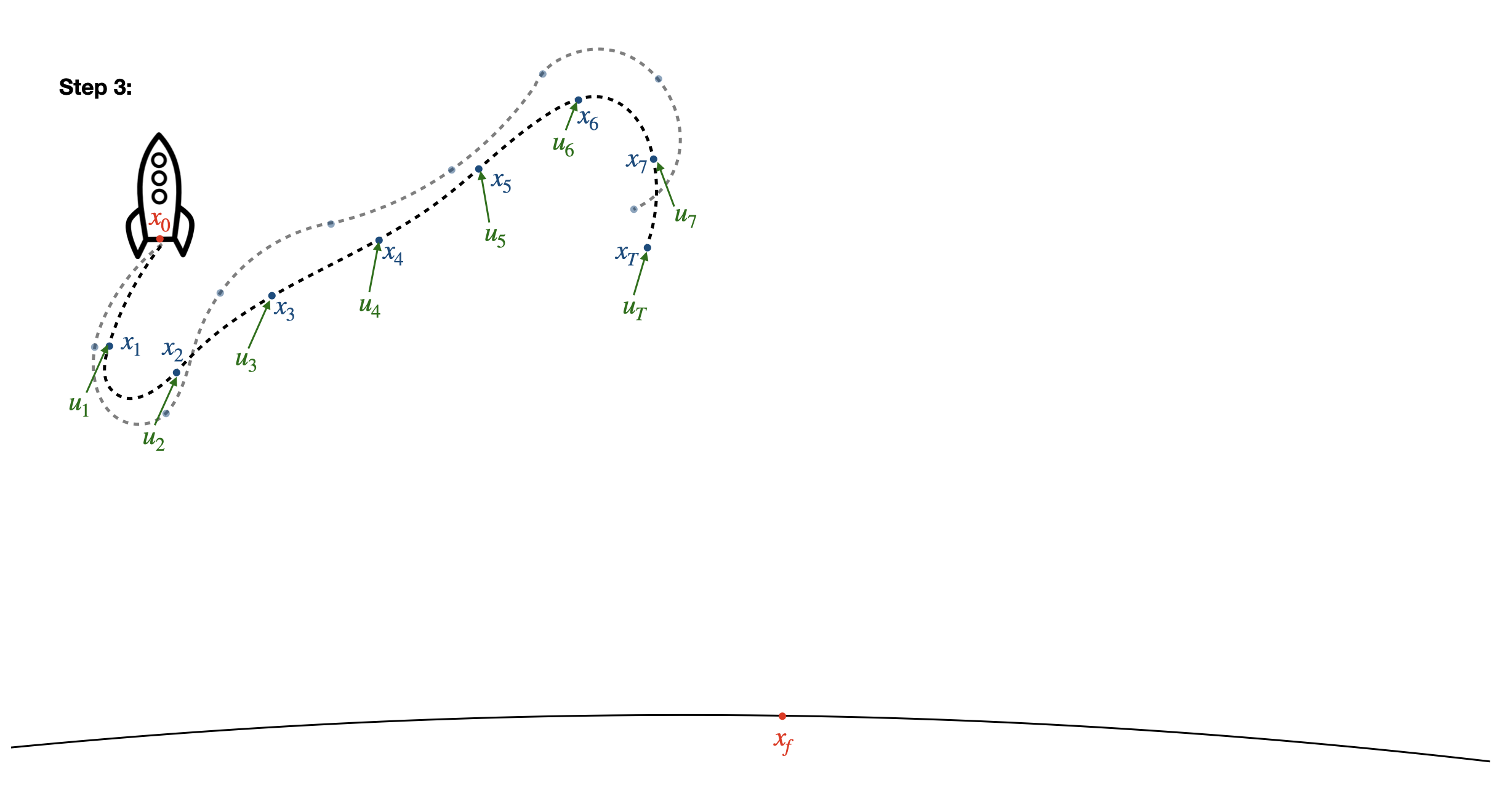
4. Repeat from step 1: apply your new \(u\) to the dynamics, linearize around this new trajectory, and optimize!
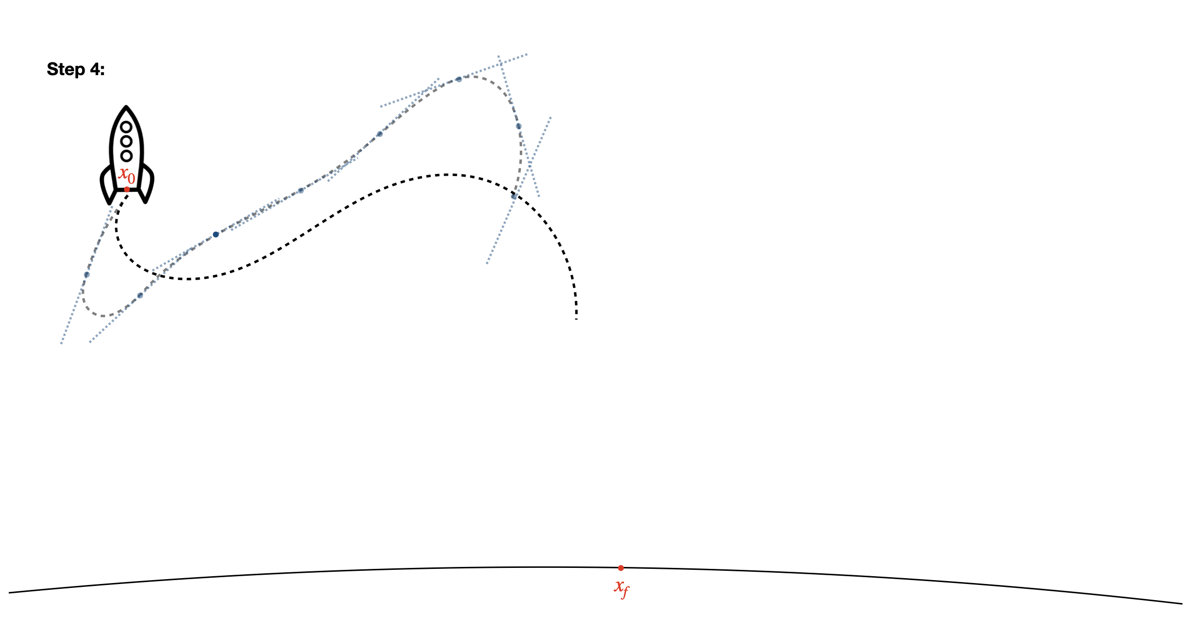
5. Repeat this process until your final state is reached within some tolerance. You now have a set of states \(x\) and inputs \(u\) that you know your rocket can follow that will get you to the landing site!

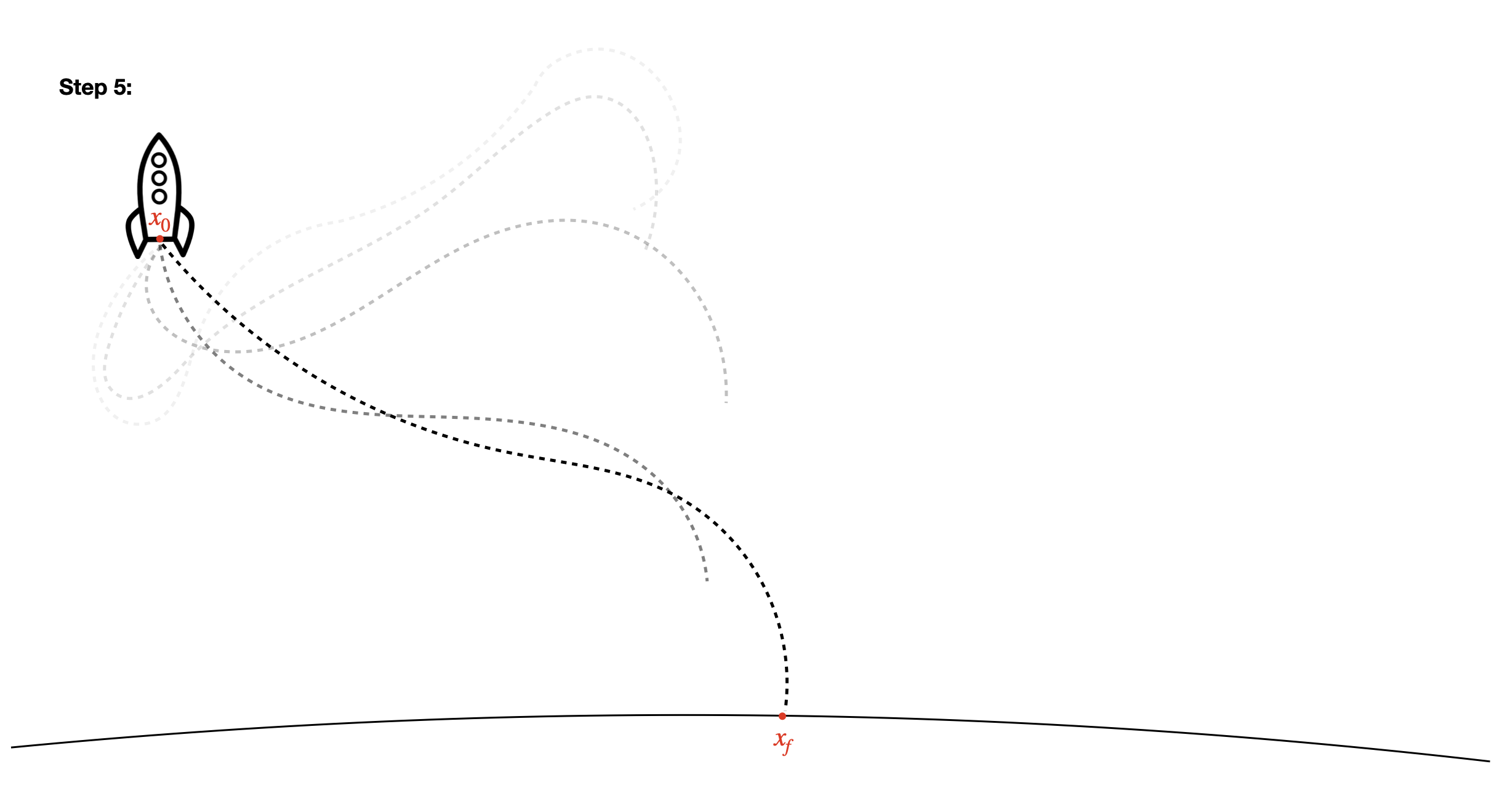
These 5 steps are all it takes to generate trajectories for complex nonlinear problems - the engineer plugs in the initial position of the rocket, a model of the dynamics, and a metric to optimize against, and SCP spits out a list of feasible control inputs to execute to achieve your goal.⁸

3.3. Rocket Landing Example

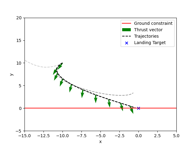
Let’s return to our rocket example, and simulate this process. To add some interesting nonlinearity, we simulate mass expenditure due to fuel use, yielding the following \(f(x,u)\):

\[\begin{bmatrix} x_{k+1} \\ y_{k+1} \\ \dot{x}_{k+1} \\ \dot{y}_{k+1} \\ m_{k+1}\end{bmatrix} = \begin{bmatrix} \dot{x}_k \Delta t \\ \dot{y}_k\Delta t \\ \frac{u_{x,k}}{m_k} \Delta t \\ (\frac{u_{y,k}}{m_k} - g) \Delta t \\ -\alpha ||u||_2 \Delta t\end{bmatrix}\]

We’ve chosen only convex constraints, except for equation \((*)\). Luckily, though, the linearization trick solves this for us and approximates it as a convex function so we can optimize it easily. Putting this into code with nonzero initial velocity, we get the following plot:

4. Practical Challenges with SCP

What challenges arise when this simple strategy is actually used in practice?

4.1. Limited Computation Resources

As you might imagine, despite huge advances in hardware and algorithms over the past several decades, this process is often still too computationally intensive to run in real-time. Instead, SCP is used to generate a trajectory (either before the launch or once at the start of a mission phase), and the spacecraft uses a simpler method (i.e. PID, LQR, MPC) to track the optimal, feasible trajectory it has been given.⁹

Think about the difference between solving a maze for the first time, and tracing a correct path someone has shown you with your pencil. If we can invest some effort into coming up with a path through the maze, all we have to do later is follow the path we’ve laid out, saving us critical computation time onboard our spacecraft.

4.2. Limited Information

When tracking a trajectory from SCP, our performance often depends directly on how well we know the position of our spacecraft. Especially when landing on the moon, this information may be not be accurate. This problem has enough complexity to be a full-fledged subfield of GN&C, and the ways in which controls and estimation interact are often subtle and unintuitive. Having a good understanding of this interplay is critical to the performance of these algorithms in flight.

4.3. Non-convex Constraints

In the same way that SCP handles non-linear dynamics, it can only handle non-convex constraints via linearization (unless you can “convexify” the constraints with some clever modifications).⁵ This means that such constraints are less likely to be satisfied. Other useful cases may be even more challenging - for example, a constraint where an engine can either be completely off or firing at some minimum thrust level is nonconvex and discontinuous, and must be handled with special care.

4.4. Hardware Failures

During the SLIM mission, one of the two main engines failed at 150 feet above the ground. This is obviously an extreme case, but highlights an important limitation of SCP - these trajectories are often generated assuming a given vehicle configuration. How robust can we make these trajectories to hardware failures? This could be handled by simply regenerating a trajectory when a actuator fails, but also potentially by adding robustness into the optimization process itself.

The issue of robustness is perhaps the most challenging (How do we define robustness? Which failures do we consider?), but also has the most potential for impact. As mission cadence increases and we begin to put human lives on the line, having robustness deeply baked into the algorithms will be critical.

5. Summary

Landing on planetary bodies is hard, and as we’ve observed recently, GN&C is often the limiting factor. In this post, I tried to provide the surprisingly simple intuition behind SCP and the ways it can seemingly magically solve difficult problems with blinding speed. If you’re interested in landing rockets, I’d urge you to play around with the code and get a feel for the power and limitations of these methods - to become an interplanetary species, there is still much work to be done in this area.

Many thanks to Sam Buckner for consulting on this post - The University of Washington has some of the world’s foremost researchers on this topic. For a more rigorous introduction to SCP (and lossless convexification, which I didn’t cover in this post), I would recommend this fantastic tutorial article.

1. Note that while I’ve worked on GN&C control software on the Orion spacecraft at NASA and for satellites at SpaceX, I’ve never worked directly on the landing problem at SpaceX or any other company. As such, take this information with a grain of salt. ↩

2. OK, I said “relatively”… ↩

3. Note that this means vertical AND horizontal velocity, and zero means ZERO. Intuitive Machines had ~2 mph crossrange velocity, and it resulted in the lander tipping over. ↩

4. And that we can take the derivative of it. Importantly, this means that things get way harder if \(f(x,u)\) is just a simulation, rather than a mathematical equation. ↩

5. Of course, a real and useful rocket landing problem might have more constraints, including minimum thrust requirements, glidescope position constraints, gimbaling limits, etc. - see the seminal G-FOLD paper. Things get more complicated in these cases, but the procedure doesn’t fundamentally change (as long as your constraints aren’t too nasty). ↩ ↩²

6. Convex Optimization by Boyd and Vandenberghe is the classic reference on the subject, but it can be quite dense. ↩

7. The quality of this approximation depends on the extent of your nonlinearities and your starting trajectory. One approach to find a more globally optimal solution is to run SCP multiple times, each with a new guess for the initial control sequence. ↩

8. I’m of course brushing over HOW to solve these optimization problems here. Luckily, in 2024 we have access to CVX and other libraries which largely abstract these lower level problems away, so we can focus on the bigger picture. See the linked code or the CVX documentation for an example of how to write these optimization problems in Python or Matlab. ↩

9. Depending on your computational resources and the speed of your dynamics, you may be able to get away with running SCP on-board in real time. You can also consider re-running SCP any time your spacecraft gets too far off course - there are infinite varieties of ways you can design your EDL system. ↩